Overview
fragquaxi allows you to obtain fractional abundances of glycoforms (and proteoforms in general) from mass spectrometric (MS) data by quantification via XIC (extracted ion current) integration.
Installation
fragquaxi is currently only available from GitHub.
remotes::install_github("cdl-biosimilars/fragquaxi")Usage
Load mass spectrometric data.
library(fragquaxi)
library(tibble)
library(dplyr)
library(tidyr)
library(ggplot2)

ms_data <- mzR::openMSfile(
  system.file("extdata", "mzml", "mab1.mzML", package = "fragquaxi")
)
Define proteins.
mab_sequence <- system.file(
  "extdata", "mab_sequence.fasta",
  package = "fragquaxi"
)

proteins <- define_proteins(
  mab = mab_sequence,
  .disulfides = 16
)
Define PTM compositions.
modcoms <- tribble(
  ~modcom_name, ~Hex, ~HexNAc, ~Fuc,
  "G0F/G0",        6,       8,    1,
  "G0F/G0F",       6,       8,    2,
  "G0F/G1F",       7,       8,    2,
  "G1F/G1F",       8,       8,    2,
  "G1F/G2F",       9,       8,    2,
  "G2F/G2F",      10,       8,    2,
) %>%
  define_ptm_compositions()
Assemble proteoforms and calculate mass-to-charge ratios of proteoform ions in charge states 33+ to 40+
pfm_ions <-
  assemble_proteoforms(proteins, modcoms) %>%
  ionize(charge_states = 33L:40L)

pfm_ions
#> # A tibble: 48 x 8
#>    protein_name modcom_name formula                         mass     z    mz
#>    <chr>        <chr>       <mol>                          <dbl> <int> <dbl>
#>  1 mab          G0F/G0      C6570 H10124 N1714 O2088 S44 147942.    33 4484.
#>  2 mab          G0F/G0      C6570 H10124 N1714 O2088 S44 147942.    34 4352.
#>  3 mab          G0F/G0      C6570 H10124 N1714 O2088 S44 147942.    35 4228.
#>  4 mab          G0F/G0      C6570 H10124 N1714 O2088 S44 147942.    36 4111.
#>  5 mab          G0F/G0      C6570 H10124 N1714 O2088 S44 147942.    37 3999.
#>  6 mab          G0F/G0      C6570 H10124 N1714 O2088 S44 147942.    38 3894.
#>  7 mab          G0F/G0      C6570 H10124 N1714 O2088 S44 147942.    39 3794.
#>  8 mab          G0F/G0      C6570 H10124 N1714 O2088 S44 147942.    40 3700.
#>  9 mab          G0F/G0F     C6576 H10134 N1714 O2092 S44 148088.    33 4489.
#> 10 mab          G0F/G0F     C6576 H10134 N1714 O2092 S44 148088.    34 4357.
#> # … with 38 more rows, and 2 more variables: mz_min <dbl>, mz_max <dbl>
Plot these ions (here, only charge state 36+ of scans 126 to 136).
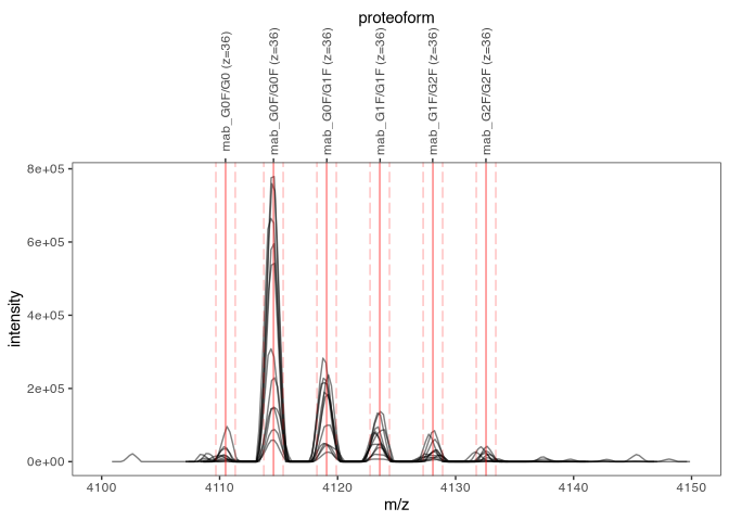
Quantify these ions via XIC integration.
abundances <- quantify_ions(
ms_data,
pfm_ions,
rt_limits = c(300, 350)
)
abundances
#> ℹ Abundances of 48 ions quantified in 352 mass spectra using 1 retention time window.
#>
#> ── Parameters ──
#>
#> MS data file:
#> '/home/wolfgang/R/x86_64-pc-linux-gnu-library/4.0/fragquaxi/extdata/mzml/mab1.mzML'
#>
#> Ions:
#> # A tibble: 48 x 9
#> ion_id protein_name modcom_name formula mass z
#> <chr> <chr> <chr> <mol> <dbl> <int>
#> 1 id_1 mab G0F/G0 C6570 H10124 N1714 O2088 S44 147942. 33
#> 2 id_2 mab G0F/G0 C6570 H10124 N1714 O2088 S44 147942. 34
#> 3 id_3 mab G0F/G0 C6570 H10124 N1714 O2088 S44 147942. 35
#> 4 id_4 mab G0F/G0 C6570 H10124 N1714 O2088 S44 147942. 36
#> 5 id_5 mab G0F/G0 C6570 H10124 N1714 O2088 S44 147942. 37
#> # … with 43 more rows, and 3 more variables: mz <dbl>, mz_min <dbl>,
#> # mz_max <dbl>
#>
#> Retention time limits:
#> # A tibble: 1 x 3
#> rt_min rt_max scans
#> <dbl> <dbl> <list>
#> 1 300 350 <int [25]>
#>
#> ── Results ──
#>
#> # A tibble: 1 x 50
#> rt_min rt_max id_1 id_2 id_3 id_4 id_5 id_6 id_7 id_8 id_9
#> <dbl> <dbl> <dbl> <dbl> <dbl> <dbl> <dbl> <dbl> <dbl> <dbl> <dbl>
#> 1 300 350 153744. 204512. 2.57e5 3.34e5 1.84e5 1.77e5 1.21e5 1.14e5 2.90e6
#> # … with 39 more variables: id_10 <dbl>, id_11 <dbl>, id_12 <dbl>, id_13 <dbl>,
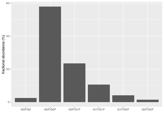
#> # id_14 <dbl>, …Plot abundances.
abundances %>%
  as_tibble() %>%
  unnest(abundance_data) %>%
  group_by(modcom_name) %>%
  summarise(abundance = sum(abundance)) %>%
  mutate(frac_ab = abundance / sum(abundance) * 100) %>%
  ggplot(aes(modcom_name, frac_ab)) +
  geom_col() +
  xlab("") +
  ylab("fractional abundance (%)")