Diagnostic plot for selecting optimal peak integration boundaries.

This function draws proteoform abundances vs the PPM value used by ionize(), which in turn determines the integration boundaries for each ion.

plot_optimal_ppm(
  ms_data,
  proteoforms,
  charge_states,
  ppm_values = seq(0, 2500, 50),
  rt_limits = c(-Inf, +Inf),
  subplots = c("all", "total", "modcom")
)

Arguments

ms_data	Mass spectrometry data stored in an mzR object as returned by mzR::openMSfile().
proteoforms	Proteoform masses as returned by assemble_proteoforms().
charge_states	Vector of charge states in which the proteoforms should be quantified.
ppm_values	Vectors of PPM values where abundances should be sampled.
rt_limits	A specification of retention time limits, passed to quantify_ions().
subplots	Subplots that should be drawn; one of "all" (draw all subplots), "total" (draw only the total abundance plot), and "modcom" (draw only the subplot with individual proteoform abundances).

Value

A ggplot object describing the created plot.

Details

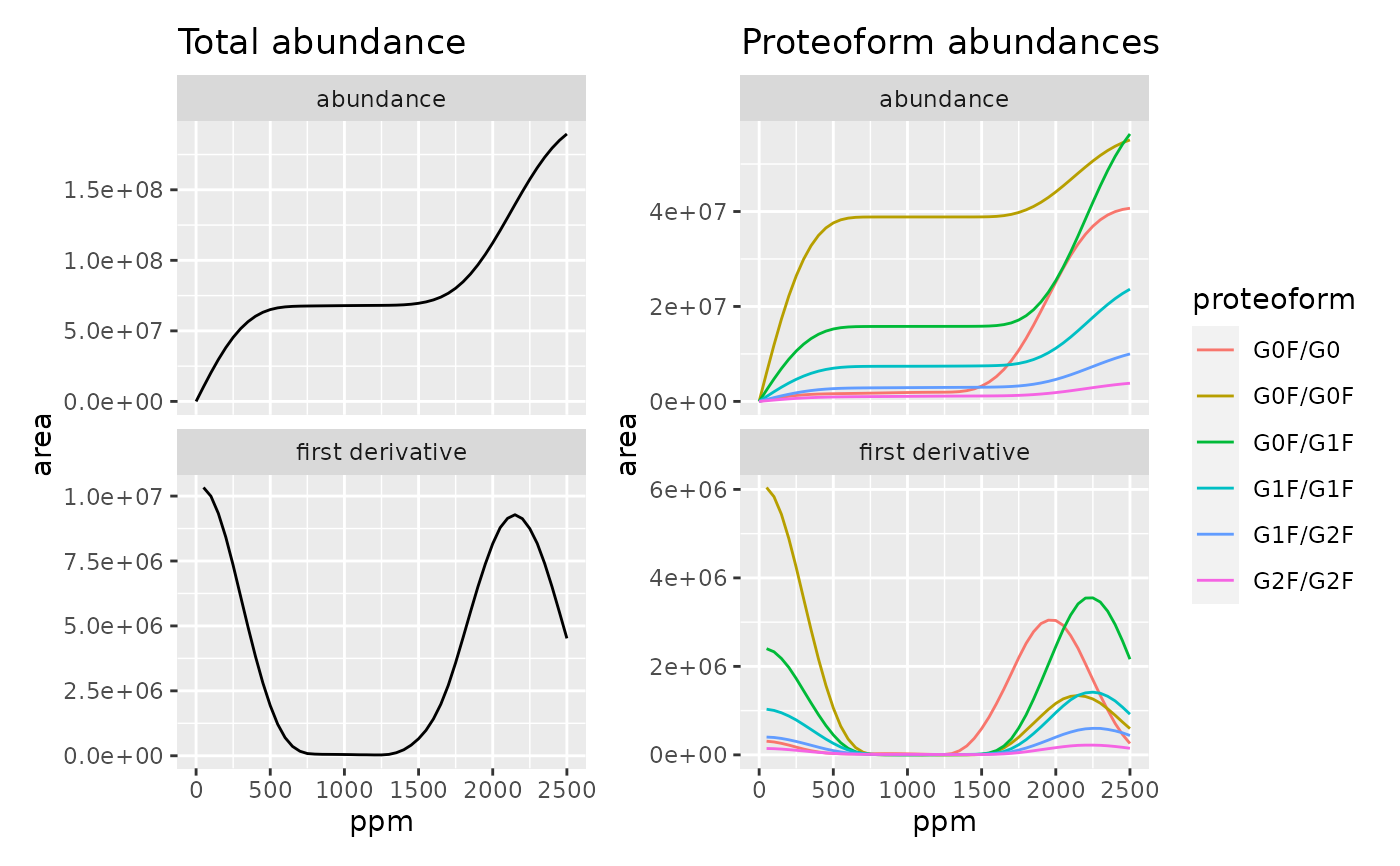
By default, the function creates four plots: Total proteoform abundance vs PPM (upper left), first derivative of this curve (lower left), individual proteoform abundances vs PPM (upper right) and first derivative of the latter curve (lower right).

Optimal integration boundaries capture each peak completely and do not lead to overlaps with neighboring peaks. This corresponds to the PPM value where the curves in the upper plots reach the first plateau, and their derivatives become zero.

Examples

ms_data <- mzR::openMSfile(
  system.file("extdata", "mzml", "mab1.mzML", package = "fragquaxi")
)
proteins <- define_proteins(
  system.file("extdata", "mab_sequence.fasta", package = "fragquaxi"),
  .disulfides = 16
)
modcoms <- define_ptm_compositions(sample_modcoms)
pfm_masses <- assemble_proteoforms(proteins, modcoms)

plot_optimal_ppm(ms_data, pfm_masses,
                 charge_states = 33L:40L, rt_limits = c(300,350))